Maternal smoking and twin infant mortality#

This notebook analyzes real birth records. It asks a perinatal question, defines the effect that answers it, and estimates that effect with targeted maximum likelihood estimation (TMLE). It then checks what the data can check, and states what they cannot.

The situation#

A perinatal epidemiologist plans a smoking-cessation program for women who carry twins. The program needs the number of infant deaths that smoking causes among twins of smoking mothers. The data are US birth certificates of same-sex twin pairs born alive in 1989–1991. The National Center for Health Statistics (NCHS) linked each birth to any infant death before the first birthday.

element	in this analysis
unit	one twin pair. The mother’s smoking and her recorded background apply to both twins
treatment A	tobacco use during the pregnancy, as the birth certificate records it
outcome Y	the share of the two twins who die before their first birthday: 0, 0.5, or 1
covariates C	background and medical history recorded on the certificate, listed below the graph
time order	most of C exists before the pregnancy. A occurs during the pregnancy. The twins are born, and Y follows over one year
observed	A, C, and Y for each pair
counterfactual	Y⁰, the share of the twins who would die if the mother did not smoke. It is observed only for the pairs with A = 0

Every pair has two children, so the mean of Y over pairs equals the first-year risk per child. The analysis reports risks per child. It treats the pair as the unit, because the twins share A and C and their outcomes are dependent.

The causal graph#

   C ─────────────┬──────────────┐
   │              │              │
   ▼              ▼              ▼
   A ──────────▶  M  ─────────▶  Y
   │              ▲              ▲
   │              U ─────────────┤
   └─────────────────────────────┘

node	what it represents	role
C	the covariates in the next table	confounders
A	tobacco use during the pregnancy	treatment
M	gestational age and birth weight of each twin, and complications of this pregnancy	mediators
U	unmeasured causes of preterm birth and low birth weight, such as birth defects	common cause of M and Y
Y	the share of the twins who die in the first year	outcome

group of C	variables	timing
mother	age, education, race, Hispanic origin, birthplace region, marital status	before the pregnancy
father	age, education	before the pregnancy
place and time	residence region, birth year	before the pregnancy
pregnancy history	total birth order, a previous preterm or small infant, a previous infant over 4,000 g	before the pregnancy
medical history	chronic hypertension; diabetes; lung, heart, or kidney disease	mostly before the pregnancy. The diabetes and lung items can include conditions that start in the pregnancy
behavior	alcohol use in the pregnancy	during the pregnancy

arrow or absent arrow	what it asserts
C → A	background and medical history change the chance that a mother smokes. Section 3 shows this for marital status and education
C → Y	the same factors change infant mortality
C → M	chronic conditions and maternal age can change gestation and fetal growth
A → M	smoking lowers birth weight and can shorten gestation
M → Y	preterm birth and low birth weight raise mortality
A → Y	smoking can affect mortality through paths outside M
U → M, U → Y	causes such as birth defects lower birth weight and raise mortality
no U → A	the unmeasured causes of low birth weight do not cause smoking
no A → C	smoking does not change any variable of C. Section 10 checks the three items for which this is doubtful
no other arrow into both A and Y	C contains every common cause of smoking and mortality. This is the main judgment of the analysis

C blocks every back-door path from A to Y, so adjustment for C identifies the total effect of A. Adjustment for M would remove the part of the effect that passes through M. It would also open the path A → M ← U → Y, because M is a collider on that path. Section 7 shows the consequence in the data. Smoking can itself cause some birth defects. The collider argument concerns the causes of U that smoking does not affect.

The analysis treats alcohol use as a marker of shared behavioral causes, which is a judgment. If smoking changes alcohol use, diabetes, or lung disease in the pregnancy, adjustment for them removes part of the effect. The analysis omits prenatal care, because care during the pregnancy can be a confounder or a mediator.

The graph leaves three points open. It has no censoring node, because the linked file records every death before the first birthday. It does not draw two selections. The cohort holds only pregnancies that end in two live births, and the source removed the pairs with equal birth weights, which is a selection on M. If smoking changes fetal survival or birth weight, these selections can bias the effect, and these data cannot measure the bias.

The question and the estimand#

Question. Among twin pregnancies in which the mother smoked, how much higher was the first-year mortality of the twins than it would have been if she had not smoked?

element	definition
target population	same-sex twin pairs born alive in the US in 1989–1991 to smoking mothers, in a residence state and year that collected the tobacco item
intervention	no tobacco use during the pregnancy, against the observed smoking
counterfactual outcome	Y⁰, the share of the twins who would die with no smoking
estimand	the average treatment effect on the treated, ATT = E[Y \| A = 1] − E[Y⁰ \| A = 1]

The ATT answers the program’s question, because a cessation program acts on mothers who smoke. The average treatment effect (ATE) would also average over non-smoking mothers. For them, “smoke” is not an intervention that anyone proposes. The crude difference E[Y | A = 1] − E[Y | A = 0] replaces E[Y⁰ | A = 1] with the risk of the non-smoking pairs. That replacement is valid only if the two groups have the same risk without smoking. Section 3 shows that they do not.

assumption	statement	how it can be assessed
no unmeasured confounding	Y⁰ is independent of A given C	scientific judgment. Section 9 measures how strong a missed confounder must be to change the answer
consistency	Y = Y⁰ for the pairs with A = 0	scientific judgment. “No smoking” has several real versions, such as never smoking or quitting early
correct exposure record	the certificate records smoking correctly	scientific judgment. The data contain no second measure of smoking
no effect of A on C	smoking does not change a variable of C	scientific judgment. Section 10 refits without the three doubtful items
positivity	P(A = 0 \| C) > 0 for the background of every smoking mother	partly checkable. Section 8 reads the fitted propensity
independent units	the outcomes of different pairs are independent	scientific judgment. The analysis does not need independence of the two twins
selection	the restrictions to live-born pairs, to unequal birth weights, and to a stated smoking status do not bias the effect	scientific judgment. Section 2 counts only the state-year and missing-item exclusions, because the source contains no other pairs

Why this method#

TMLE estimates the ATT from two nuisance models. The outcome regression is E(Y | A, C). The propensity is P(A = 1 | C). TMLE fits both. It then updates the outcome regression so that the estimate solves the efficient influence-curve equation of the ATT. Each method choice below follows from a feature of this problem.

feature of the problem	method choice
18 covariates, most of them categorical, with unknown interactions	a Super Learner for each nuisance: a main-terms logistic model and a gradient-boosting model, weighted by cross-validation
the boosting model adapts to the data	cross-fitting over three folds. Each nuisance prediction comes from models fit on the other folds, so the analysis needs no Donsker condition on the learners. The product of the two nuisance errors must still shrink faster than n^(-1/2)
the outcome is a share in [0, 1]	a logistic fluctuation with `q_bounds=(0, 1)`, which keeps every estimate in the outcome’s range
either nuisance model can be wrong	the estimate is consistent if either nuisance model is consistent
the outcome is rare, so the outcome model explains little	the estimator then behaves close to inverse-probability weighting, and the propensity drives its precision
the target is the ATT	the update weights a non-smoking pair by g/(1 − g), with g its propensity. Overlap is needed only where the smoking mothers are
the pair is the unit	one row per pair, so the influence-curve standard error needs no cluster correction

term	meaning
nuisance	a model that the estimate needs and the question does not ask about
propensity g(C)	P(A = 1 \| C), the probability that the mother smokes given her background
targeting	the update of the outcome regression that removes the first-order bias of the plug-in estimate
influence curve	the contribution of each pair to the estimate. Its variance gives the standard error
Super Learner	a weighted combination of candidate learners, with weights from cross-validation

1. Setup#

The data step downloads three CSV files, so the notebook needs a network connection.

import platform

import matplotlib.pyplot as plt
import numpy as np
import pandas as pd
import sklearn
from sklearn.ensemble import HistGradientBoostingClassifier, HistGradientBoostingRegressor
from sklearn.linear_model import LogisticRegression

import cleverly
from cleverly import (
    ATT,
    CausalStudy,
    CrossFitting,
    Inference,
    ModelSpec,
    PointTreatment,
    Runtime,
    StudyProtocol,
    SuperLearner,
    Targeting,
    TMLEMethod,
)
from cleverly.learners import GLM

SEED = 2026
pd.set_option("display.width", 120)
print("python", platform.python_version())
print("cleverly", cleverly.__version__)
print("numpy", np.__version__, "| pandas", pd.__version__, "| scikit-learn", sklearn.__version__)

python 3.13.16
cleverly 0.1.3
numpy 2.5.4 | pandas 3.0.6 | scikit-learn 1.9.1

What this output tells you. The stored outputs came from these versions. Another version can print other numbers.

2. Build the cohort#

The files come from the TWINS extraction of Louizos et al. (2017), pinned to one commit of the CEVAE repository. That extraction holds the same-sex twin pairs of the NCHS linked files for 1989–1991, without the pairs with equal birth weights. NCHS collected the data. NCHS is not responsible for this analysis or its conclusions. The references give the data-use rules.

Some states did not collect the tobacco item in some years. The NCHS guides name them: California, Indiana, New York, and South Dakota in all three years, Oklahoma in 1989 and 1990, and Louisiana and Nebraska in 1989. The code keeps a state-year when at most half of its pairs lack the item. It then drops the pairs whose item is not stated.

The code keeps the variables of C at their recorded levels, and it pools sparse levels with their neighbors. A missing categorical value becomes the level “not recorded”. The seven medical risk-factor items are missing together, so one indicator, risk_factors_recorded, marks those pairs.

COMMIT = "9081f863e24ce21bd34c8d6a41bf0edc7d1b65dd"
BASE_URL = f"https://raw.githubusercontent.com/AMLab-Amsterdam/CEVAE/{COMMIT}/datasets/TWINS"
raw = {
    name: pd.read_csv(f"{BASE_URL}/twin_pairs_{name}_3years_samesex.csv")
    for name in ("X", "T", "Y")
}
X, T, Y = raw["X"], raw["T"], raw["Y"]
assert len(X) == len(T) == len(Y)

# Some residence states did not collect the tobacco item in some years. Keep the state-years
# that did: in those, at most half of the pairs lack the item.
state_year = [X["brstate"], X["data_year"]]
missing_share = X["tobacco"].isna().groupby(state_year).transform("mean")
reporting_state = missing_share <= 0.5
eligible = reporting_state & X["tobacco"].notna()


def category(column, merge=None):
    """A covariate as string levels. Missing values form the level "not recorded"."""
    values = X.loc[eligible, column].map(lambda value: merge.get(value, value) if merge else value)
    labels = values.map(lambda value: "not recorded" if pd.isna(value) else str(int(value)))
    return labels.to_numpy()


source = X.loc[eligible]
# The seven medical risk-factor items are missing together, so one indicator records that.
risk_items = ["diabetes", "chyper", "lung", "cardiac", "renal", "preterm", "pre4000"]
risk_missing = source[risk_items].isna()
assert risk_missing.eq(risk_missing["diabetes"], axis=0).all(axis=None)
risk = source[risk_items].fillna(0).astype(float)

pairs = pd.DataFrame(
    {
        "smoked": source["tobacco"].astype(int).to_numpy(),
        "death_share": (Y.loc[eligible, "mort_0"] + Y.loc[eligible, "mort_1"]).to_numpy() / 2,
        # Sparse levels are pooled with their neighbours.
        "mother_age": category("mager8", {1: 2, 8: 7}),
        "mother_education": category("meduc6"),
        "father_education": category("feduc6"),
        "father_age": category("dfageq"),
        "mother_race": category("mrace", dict.fromkeys(range(4, 10), 3)),
        "mother_hispanic": category("ormoth", dict.fromkeys(range(2, 6), 1)),
        "mother_birth_region": category("mplbir_reg"),
        "residence_region": category("brstate_reg"),
        "birth_year": category("data_year"),
        "birth_order": category("dtotord_min", dict.fromkeys(range(6, 40), 5)),
        "married": source["dmar"].astype(float).to_numpy(),
        "alcohol": category("alcohol"),
        "risk_factors_recorded": 1.0 - risk_missing["diabetes"].astype(float).to_numpy(),
        "diabetes": risk["diabetes"].to_numpy(),
        "chronic_hypertension": risk["chyper"].to_numpy(),
        "lung_heart_kidney_disease": risk[["lung", "cardiac", "renal"]].max(axis=1).to_numpy(),
        "previous_preterm_or_small": risk["preterm"].to_numpy(),
        "previous_infant_over_4000g": risk["pre4000"].to_numpy(),
    }
)
ADJUSTMENT = tuple(column for column in pairs.columns if column not in ("smoked", "death_share"))

print(f"pairs in the source file:              {len(X):,}")
print(f"pairs in state-years without the item: {(~reporting_state).sum():,}")
print(f"pairs with the item not stated:        {(reporting_state & X['tobacco'].isna()).sum():,}")
print(f"eligible pairs:                        {len(pairs):,}")
print(f"pairs with smoking recorded:           {pairs['smoked'].mean():.4f}")
print(f"first-year mortality per child:        {pairs['death_share'].mean():.4f}")
print(f"adjustment variables:                  {len(ADJUSTMENT)}")
print()
print("excluded state-years: residence-state code, birth years, pairs")
excluded = X.loc[~reporting_state].groupby("brstate")
for code, group in excluded:
    years = ", ".join(str(1900 + year) for year in sorted(group["data_year"].unique()))
    print(f"  {code:>2}  {years:<16}  {len(group):>5,}")

pairs in the source file:              71,345
pairs in state-years without the item: 16,739
pairs with the item not stated:        2,732
eligible pairs:                        51,874
pairs with smoking recorded:           0.1628
first-year mortality per child:        0.0361
adjustment variables:                  18

excluded state-years: residence-state code, birth years, pairs
   5  1989, 1990, 1991  8,536
  15  1989, 1990, 1991  1,535
  19  1989                464
  28  1989                188
  33  1989, 1990, 1991  5,315
  37  1989, 1990          489
  42  1989, 1990, 1991    209
  52  1991                  1
  55  1989                  2

What this output tells you. The source file holds 71,345 pairs. The state-years without the item hold 16,739 pairs. Their residence-state codes are the states that the guides name: 5 (California), 15 (Indiana), 19 (Louisiana), 28 (Nebraska), 33 (New York), 37 (Oklahoma), and 42 (South Dakota). Code 52 holds 1 pair in 1991, and code 55 holds 2 pairs in 1989.

In the kept state-years, 2,732 pairs have no stated smoking status. The cohort holds 51,874 pairs. Smoking is recorded for a share of 0.1628 of them. The first-year mortality is 0.0361 per child.

The estimate therefore describes the twin births of the reporting states and years. It assumes that the removal of the pairs with no stated smoking status does not bias the effect.

3. The crude association, and why it is confounded#

The crude difference uses the non-smoking pairs to stand in for E[Y⁰ | A = 1]. A covariate of C biases that stand-in when two conditions hold: its distribution differs between the groups, and it predicts mortality without smoking. The code computes the crude difference with a Wald interval over pairs. For four covariates, it then prints the share in each group and the risk of the non-smoking pairs with and without the covariate.

smoker = pairs["smoked"] == 1
risk_smoked = pairs.loc[smoker, "death_share"].mean()
risk_not = pairs.loc[~smoker, "death_share"].mean()
crude = risk_smoked - risk_not
# Pairs are the independent units, so the standard error uses the pair-level outcome.
crude_se = np.sqrt(
    pairs.loc[smoker, "death_share"].var() / smoker.sum()
    + pairs.loc[~smoker, "death_share"].var() / (~smoker).sum()
)
print(f"risk, children of smoking mothers:     {risk_smoked:.4f}")
print(f"risk, children of non-smoking mothers: {risk_not:.4f}")
crude_ci = (crude - 1.96 * crude_se, crude + 1.96 * crude_se)
print(f"crude difference: {crude:.4f}, 95% CI [{crude_ci[0]:.4f}, {crude_ci[1]:.4f}]")
print()
factors = {
    "unmarried": pairs["married"] == 0,
    "mother_education 1-2": pairs["mother_education"].isin(["1", "2"]),
    "birth_order 4+": pairs["birth_order"].isin(["4", "5"]),
    "alcohol use": pairs["alcohol"] == "1",
}
non_smoking = pairs.loc[~smoker]
imbalance = pd.DataFrame(
    {
        "share, smoking": {name: mask[smoker].mean() for name, mask in factors.items()},
        "share, non-smoking": {name: mask[~smoker].mean() for name, mask in factors.items()},
        "risk if present, non-smoking": {
            name: non_smoking.loc[mask[~smoker], "death_share"].mean()
            for name, mask in factors.items()
        },
        "risk if absent, non-smoking": {
            name: non_smoking.loc[~mask[~smoker], "death_share"].mean()
            for name, mask in factors.items()
        },
    }
)
print(imbalance.round(4).to_string())

risk, children of smoking mothers:     0.0427
risk, children of non-smoking mothers: 0.0348
crude difference: 0.0078, 95% CI [0.0038, 0.0119]

                      share, smoking  share, non-smoking  risk if present, non-smoking  risk if absent, non-smoking
unmarried                     0.4053              0.2165                        0.0588                       0.0282
mother_education 1-2          0.3216              0.1460                        0.0521                       0.0319
birth_order 4+                0.2853              0.1674                        0.0324                       0.0353
alcohol use                   0.1017              0.0119                        0.0350                       0.0348

What this output tells you. The risk is 0.0427 for the children of smoking mothers and 0.0348 for the others. The crude difference is 0.0078, with a 95% interval of [0.0038, 0.0119].

covariate	share, smoking	share, non-smoking	risk, non-smoking, with it	risk, non-smoking, without it	direction of crude bias
unmarried	0.4053	0.2165	0.0588	0.0282	upward: both conditions hold
mother’s education in the two lowest categories	0.3216	0.1460	0.0521	0.0319	upward: both conditions hold
total birth order 4 or higher	0.2853	0.1674	0.0324	0.0353	downward: more common with smoking, and the risk is lower with it
alcohol use	0.1017	0.0119	0.0350	0.0348	none visible. Few non-smoking mothers report alcohol use, so their risk is imprecise

Unmarried mothers and mothers with less education smoke more often. Without smoking, their twins also die more often. These two covariates therefore make the crude difference larger than the ATT. Birth order acts in the other direction, with a smaller risk difference. The net bias needs an analysis that adjusts for all of C together.

4. Write the protocol#

A StudyProtocol records the design before any model runs. Every result fitted from the study stores its fingerprint.

protocol = StudyProtocol(
    target_population=(
        "Same-sex twin pairs born alive in the US in 1989-1991, to mothers resident in a state "
        "that collected the tobacco item in the year of birth"
    ),
    eligibility=(
        "Both twins born alive, with unequal birth weights (the source removed equal pairs)",
        "The residence state collected the tobacco item in the year of birth",
        "Tobacco use stated for this pregnancy",
    ),
    time_zero="Birth of the twins; smoking status refers to the pregnancy before it",
    treatment_strategies=("Smoking during pregnancy, as recorded", "No smoking during pregnancy"),
    treatment_versions=(
        "Any recorded tobacco use, at any amount and in any trimester",
        "No tobacco use at any time in the pregnancy",
    ),
    outcome="Share of the two twins who die before their first birthday",
    horizon="First year after birth",
    intercurrent_event_handling=("None: the linked file records every first-year death",),
    interference_unit="Twin pair",
    assumption_rationale=(
        "Exchangeability: pre-pregnancy background and chronic conditions are adjusted; "
        "unmeasured behaviour and environment can still confound",
        "Consistency: no smoking has several real versions, such as never smoking or quitting",
        "Positivity: checked on the fitted propensity of the smoking pairs",
        "Selection: the cohort is restricted to live-born twin pairs, which smoking can affect",
    ),
)
print("\n".join(protocol.summary_lines()))

causal study protocol: schema 1; 59fee493706efdcb
target population: Same-sex twin pairs born alive in the US in 1989-1991, to mothers resident in a state that collected the tobacco item in the year of birth
eligibility: ['Both twins born alive, with unequal birth weights (the source removed equal pairs)', 'The residence state collected the tobacco item in the year of birth', 'Tobacco use stated for this pregnancy']
time zero: Birth of the twins; smoking status refers to the pregnancy before it
treatment strategies: ['Smoking during pregnancy, as recorded', 'No smoking during pregnancy']
treatment versions: ['Any recorded tobacco use, at any amount and in any trimester', 'No tobacco use at any time in the pregnancy']
outcome: Share of the two twins who die before their first birthday
horizon: First year after birth
intercurrent-event handling: ['None: the linked file records every first-year death']
interference unit: Twin pair
assumption rationale: ['Exchangeability: pre-pregnancy background and chronic conditions are adjusted; unmeasured behaviour and environment can still confound', 'Consistency: no smoking has several real versions, such as never smoking or quitting', 'Positivity: checked on the fitted propensity of the smoking pairs', 'Selection: the cohort is restricted to live-born twin pairs, which smoking can affect']

What this output tells you. The first line gives the fingerprint 59fee493706efdcb. The other lines record the population, the eligibility rules of section 2, and the two strategies. The treatment versions line states that “no smoking” means no tobacco use at any time in the pregnancy. The assumption rationale line records the four judgments of the plan.

5. Identify the ATT#

The design names the outcome, the treatment, and the adjustment set C. It declares no cluster, because each row is a pair.

study = CausalStudy(
    pairs,
    design=PointTreatment(outcome="death_share", treatment="smoked", adjustment=ADJUSTMENT),
    protocol=protocol,
)
att_effect = study.identify(ATT(reference=0))
print(att_effect.summary(protocol="fingerprint"))

average treatment effect among units receiving each comparison arm
identified by explicit-adjustment: E_{W | smoked=a}[E(death_share | smoked=a, W) - E(death_share | smoked=0, W)] for a in [1]
adjustment/history: ['mother_age', 'mother_education', 'father_education', 'father_age', 'mother_race', 'mother_hispanic', 'mother_birth_region', 'residence_region', 'birth_year', 'birth_order', 'married', 'alcohol', 'risk_factors_recorded', 'diabetes', 'chronic_hypertension', 'lung_heart_kidney_disease', 'previous_preterm_or_small', 'previous_infant_over_4000g']
required nuisances: ['outcome_regression', 'treatment_mechanism']
assumptions:
  - consistency: Y = Y^a when A = a
  - no interference: one unit's potential outcome does not depend on other units' treatment assignments
  - no unmeasured confounding: Y^a is independent of A given W
  - positivity for the reference arm within each comparison population: P(smoked = 0 | W) > 0 wherever P(smoked = a | W) > 0, for every comparison arm a
  - the conditioning event has positive probability: P(smoked = a) > 0 for every comparison arm a
causal study protocol: schema 1; 59fee493706efdcb

What this output tells you. The first line names the estimand: the effect among the units that received the comparison arm. The second line is the identifying formula. It averages E(Y | A = 1, C) − E(Y | A = 0, C) over the covariates of the smoking pairs. The adjustment list holds the 18 variables of C. The assumptions are the library’s generic list. The plan states which of them need scientific judgment.

6. Estimate the ATT#

The method uses the choices of the plan. The outcome learner combines a quasi-binomial generalized linear model (GLM(family="binomial"), a logistic model for a share) and a gradient-boosting model with a Poisson loss. The treatment learner combines a logistic model and a gradient-boosting classifier. Both boosting models are regularized and limited in depth. The classifier stops early on a validation split.

def outcome_library():
    return SuperLearner(
        library=[
            ("quasi-binomial GLM", GLM(family="binomial")),
            (
                "boosting",
                HistGradientBoostingRegressor(
                    loss="poisson",
                    max_depth=3,
                    learning_rate=0.05,
                    max_iter=300,
                    l2_regularization=1.0,
                    random_state=SEED,
                ),
            ),
        ],
        task="regression",
        n_folds=3,
        random_state=SEED,
        n_jobs=1,
    )


def treatment_library():
    return SuperLearner(
        library=[
            ("logistic", LogisticRegression(max_iter=3_000, random_state=SEED)),
            (
                "boosting",
                HistGradientBoostingClassifier(
                    max_depth=6,
                    learning_rate=0.05,
                    max_iter=2_000,
                    l2_regularization=1.0,
                    early_stopping=True,
                    random_state=SEED,
                ),
            ),
        ],
        task="classification",
        n_folds=3,
        random_state=SEED,
        n_jobs=1,
    )


method = TMLEMethod(
    models=ModelSpec(outcome_learner=outcome_library(), treatment_learner=treatment_library()),
    cross_fitting=CrossFitting(n_folds=3, learner_folds=3),
    targeting=Targeting(q_bounds=(0.0, 1.0)),
    inference=Inference(alpha=0.05),
    runtime=Runtime(random_state=SEED, n_jobs=1),
)
result = att_effect.estimate(method=method)
att = result["att"]
print(result.summary(protocol="fingerprint"))
print()
print(f"observed risk, smoking pairs:       {risk_smoked:.4f}")
print(f"estimated risk had they not smoked: {risk_smoked - att.psi:.4f}")
print(f"risk, non-smoking pairs:            {risk_not:.4f}")
print(f"ATT: {att.psi:.4f}, 95% CI [{att.ci[0]:.4f}, {att.ci[1]:.4f}]")
print(f"crude difference: {crude:.4f}")
# The ATT is a risk per child, so the count of deaths scales it by the children of smoking pairs.
children_exposed = 2 * int(smoker.sum())
deaths = [children_exposed * value for value in (att.psi, *att.ci)]
print(
    f"deaths caused among {children_exposed:,} children: {deaths[0]:.0f}, "
    f"95% CI [{deaths[1]:.0f}, {deaths[2]:.0f}]"
)
initial = np.concatenate(list(result.nuisance.outcome.arms.values()))
print(f"initial outcome predictions: {initial.min():.4f} to {initial.max():.4f}")

Targeted maximum likelihood estimation
======================================
n = 51874; covariates = 60; P(A=1) = 0.1628
causal estimand: average treatment effect among units receiving each comparison arm
identification: explicit-adjustment; E_{W | smoked=a}[E(death_share | smoked=a, W) - E(death_share | smoked=0, W)] for a in [1]
required nuisances: outcome_regression, treatment_mechanism
identification assumptions: consistency: Y = Y^a when A = a; no interference: one unit's potential outcome does not depend on other units' treatment assignments; no unmeasured confounding: Y^a is independent of A given W; positivity for the reference arm within each comparison population: P(smoked = 0 | W) > 0 wherever P(smoked = a | W) > 0, for every comparison arm a; the conditioning event has positive probability: P(smoked = a) > 0 for every comparison arm a
causal study protocol: schema 1; 59fee493706efdcb
outcome family: gaussian; fluctuation: logistic (iterative)
stacked CV-TMLE (Levy): nuisances cross-fitted over 3 folds; targeting: pooled
propensity truncated to [0.002022, 0.998]; ATT/ATC to [0.025, 0.975]
data 90266a93ad1c74e7 | folds 2e17bcad9ec0a91b | cleverly 0.1.3 | 2026-10-16T01:18:19+00:00

estimand  psi        std_err   95% CI                   p_value
--------  ---------  --------  -----------------------  -------
att       0.0014499  0.002637  [-0.0037179, 0.0066176]  0.5824 

observed risk, smoking pairs:       0.0427
estimated risk had they not smoked: 0.0412
risk, non-smoking pairs:            0.0348
ATT: 0.0014, 95% CI [-0.0037, 0.0066]
crude difference: 0.0078
deaths caused among 16,888 children: 24, 95% CI [-63, 112]
initial outcome predictions: 0.0099 to 0.4709

What this output tells you. The line stacked CV-TMLE (Levy) confirms three-fold cross-fitting. The line outcome family: gaussian means that the library treats the share as a continuous outcome, because the share takes the value 0.5. With the declared range [0, 1] and the logistic fluctuation, the fit is TMLE for a bounded continuous outcome. The initial outcome predictions lie between 0.0099 and 0.4709, inside that range. The ATT is 0.0014, with a 95% influence-curve interval of [-0.0037, 0.0066].

quantity	value	source
observed risk, smoking pairs	0.0427	E[Y \| A = 1], from the data
estimated risk had they not smoked	0.0412	E[Y⁰ \| A = 1], the observed risk minus the ATT
risk, non-smoking pairs	0.0348	E[Y \| A = 0], the crude stand-in
ATT	0.0014	the adjusted estimate
crude difference	0.0078	section 3

The 16,888 children of smoking pairs give the ATT a count scale. The estimate is 24 deaths caused by smoking, with a 95% interval from -63 to 112.

The crude difference and the ATT share the observed risk of the smoking pairs. They differ only in the comparison risk. Adjustment for C moves that risk from 0.0348 to 0.0412. The ATT compares smoking mothers with non-smoking mothers of the same recorded background. The gap between 0.0078 and 0.0014 estimates the confounding by C. Its direction is the one that section 3 predicts, and its size is uncertain, because both numbers carry sampling error.

7. Why the adjustment set stops before birth weight#

Birth weight predicts infant mortality strongly, so adjustment for it can seem natural. The graph says that it is wrong for this question. Birth weight is a mediator (A → M), so adjustment for it removes part of the effect. It is also a collider on A → M ← U → Y. Within a birth-weight band, a low weight in a non-smoking pregnancy points more often to another cause, such as a birth defect, and that cause raises mortality. Hernández-Díaz, Schisterman and Hernán (2006) give this explanation of the “birth-weight paradox” in their Figure 3.

The code tabulates the first-year risk of each child by birth-weight band and smoking. These are stratum-specific associations. They do not estimate an effect of smoking, and no estimator fit within the bands would target the ATT.

children = pd.DataFrame(
    {
        "smoked": np.tile(pairs["smoked"].to_numpy(), 2),
        "birth_weight_g": np.concatenate(
            [T.loc[eligible, f"dbirwt_{twin}"].to_numpy() for twin in (0, 1)]
        ),
        "died": np.concatenate([Y.loc[eligible, f"mort_{twin}"].to_numpy() for twin in (0, 1)]),
    }
)
BANDS = [0, 1_500, 2_000, 2_500, 3_000, 10_000]
BAND_LABELS = ["under 1500 g", "1500-1999 g", "2000-2499 g", "2500-2999 g", "3000 g or more"]
children["band"] = pd.cut(children["birth_weight_g"], BANDS, right=False, labels=BAND_LABELS)
by_band = children.pivot_table(
    index="band", columns="smoked", values="died", aggfunc=["mean", "size"], observed=True
)
by_band.columns = [
    "risk, non-smoking",
    "risk, smoking",
    "children, non-smoking",
    "children, smoking",
]
low_weight = children.groupby("smoked")["birth_weight_g"].apply(
    lambda weight: (weight < 2_500).mean()
)
print(f"share under 2500 g: non-smoking {low_weight.loc[0]:.4f}, smoking {low_weight.loc[1]:.4f}")
print()
print(by_band.round(4).to_string())

fig, ax = plt.subplots(figsize=(8, 4))
for column, color in (("risk, non-smoking", "#4c78a8"), ("risk, smoking", "#e45756")):
    ax.plot(BAND_LABELS, by_band[column], marker="o", color=color, label=column)
ax.set_yscale("log")
ax.set_ylabel("First-year mortality (log scale)")
ax.set_title("Within birth-weight bands, the smoking contrast changes sign")
ax.legend()
fig.tight_layout()

share under 2500 g: non-smoking 0.4972, smoking 0.6457

                risk, non-smoking  risk, smoking  children, non-smoking  children, smoking
band                                                                                      
under 1500 g               0.3050         0.2607                   7970               2106
1500-1999 g                0.0213         0.0217                  10221               3086
2000-2499 g                0.0082         0.0119                  24994               5713
2500-2999 g                0.0046         0.0065                  28369               4479
3000 g or more             0.0027         0.0053                  15306               1504

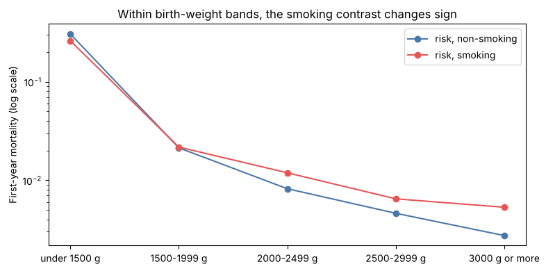
../_images/8926a3008bf4a9565e9040f9624acefedb5ab7a37bec6419476361776b5ea5ae.png

What this output tells you. In this table, a share of 0.6457 of the children of smoking mothers weigh under 2,500 g, against 0.4972 of the others. That difference agrees with the arrow A → M, although it is not adjusted for C. Within the bands, the contrast changes sign. Under 1,500 g the risk is 0.2607 with smoking and 0.3050 without it. At 3,000 g or more it is 0.0053 with smoking and 0.0027 without it. The figure shows the two curves on a log scale.

An analysis that adjusts for birth weight could conclude that smoking protects the lightest twins. The graph gives one explanation: collider bias on A → M ← U → Y. The table counts children, not pairs, and it has no intervals. It therefore supports no inference about the size of either contrast. The ATT of section 6 does not condition on M.

8. Check the fit#

result.assess() runs the validation, diagnostic, and sensitivity checks that need no refit. The code prints the status of each check that ran, the nuisance report, and the score check. These checks describe the fitted models. They cannot detect a missing confounder or an ill-defined intervention.

assessment = result.assess(random_state=SEED)
ledger = assessment.to_frame()
ran = ledger[~ledger["status"].isin(["unavailable", "not_applicable"])]
print(ran[["surface", "check", "status"]].to_string(index=False))
print("needs attention:", tuple(item.name for item in assessment.attention))
print()
print(assessment.report("nuisance_models").summary())
print()
scores = assessment.report("score_equations").to_frame()
lines = [
    f"score equation {row.name}: passed={row.passed}; |score| / threshold = {row.ratio:.4f}"
    for row in scores.itertuples()
]
# The report can list one equation in more than one row. Print each distinct line once.
print("\n".join(dict.fromkeys(lines)))

    surface                 check    status
 validation       score_equations    passed
 validation               support   warning
 validation       nuisance_models   warning
diagnostics      truncation_curve  deferred
diagnostics                refute  deferred
sensitivity   omitted_confounding   warning
sensitivity      robustness_value completed
sensitivity              elements completed
sensitivity             benchmark  deferred
sensitivity simulated_confounding  deferred
sensitivity               contour completed
sensitivity                evalue completed
needs attention: ('support', 'nuisance_models', 'omitted_confounding')

Nuisance model diagnostics
----------------------------------------
model       auc     brier   log_loss  r2      mse     cal_slope  cal_se  reg_slope
----------  ------  ------  --------  ------  ------  ---------  ------  ---------
propensity  0.7987  0.1107  0.3588    -       -       1.0731     0.0138  -        
outcome     -       -       -         0.0138  0.0272  -          -       1.0345   
Calibration slope: logistic recalibration of the out-of-fold predictions with one intercept per fold.
A finding needs the 95.0% interval to lie above 0 and exclude 1, a Bonferroni level over 1 tested model(s).

propensity: super learner weights logistic=0.366, boosting=0.634

outcome: super learner weights quasi-binomial GLM=0.555, boosting=0.445

VERDICT:
  - propensity: the out-of-fold predictions are more moderate than the observed rates (calibration slope 1.07, 95.0% interval 1.05 to 1.10, AUC 0.799, largest untruncated inverse weight 193). Review the learner before you change the model
  - the outcome model explains little variance (R^2 0.014); the estimate is close to inverse-probability weighting and will be correspondingly noisy

score equation att: passed=True; |score| / threshold = 0.0000

What this output tells you. The score equation of the ATT passed, so the targeting step solved it. Three checks need attention.

check	what it reports	reading
`nuisance_models`	a propensity calibration slope of 1.07, with an interval from 1.05 to 1.10, and an outcome R² of 0.014	a slope above 1 means that the out-of-fold propensities are slightly too moderate. The low R² is expected for a rare outcome. The estimate then relies mostly on the propensity, so the calibration of the propensity matters
`support`	12.89% of the pairs are clipped at the ATT bound	the next cell shows that this clipping does not move the estimate
`omitted_confounding`	a bound at the default strengths	section 9 reads the bound at strengths calibrated against observed covariates

The propensity flag is a prompt to review the learner. It is not a finding that the estimate is wrong. The boosting model has a weight of 0.634 in the propensity Super Learner.

print(assessment.report("support").summary())
g_hat = result.nuisance.propensity.arm(1.0)
print(f"largest fitted propensity: {g_hat.max():.4f}")
print(
    f"pairs below the lower ATT bound 0.025: non-smoking {(g_hat[~smoker] < 0.025).sum():,}, "
    f"smoking {(g_hat[smoker] < 0.025).sum():,}"
)
print()
curve = result.diagnostics.truncation_curve(bounds=(0.002, 0.005, 0.01, 0.025, 0.05))
print(
    curve[["bound", "truncated_fraction", "psi", "ci_lower", "ci_upper"]]
    .round(5)
    .to_string(index=False)
)

fig, ax = plt.subplots(figsize=(8, 4))
bins = np.linspace(0, 1, 41)
ax.hist(
    g_hat[~smoker], bins=bins, density=True, histtype="step", linewidth=2, label="non-smoking pairs"
)
ax.hist(g_hat[smoker], bins=bins, density=True, histtype="step", linewidth=2, label="smoking pairs")
ax.set_xlabel("Out-of-fold estimated P(smoked = 1 | W)")
ax.set_ylabel("Density")
ax.set_title("Fitted propensity by observed smoking status")
ax.legend()
fig.tight_layout()

Positivity / overlap diagnostics
--------------------------------
n = 51874; propensity truncated to [0.002022, 0.998]

g(W) quantile  0%      1%      5%      25%     50%     75%     95%     99%     100%  
-------------  ------  ------  ------  ------  ------  ------  ------  ------  ------
overall        0.0035  0.0111  0.0167  0.0506  0.1208  0.2191  0.4778  0.7398  0.9537
treated        0.0052  0.0228  0.0615  0.1601  0.2642  0.4261  0.7450  0.8803  0.9537
control        0.0035  0.0107  0.0160  0.0412  0.1010  0.1844  0.3781  0.5631  0.9305

arm      n      effective n  ESS / n  top 1% weight  top 5% weight
-------  -----  -----------  -------  -------------  -------------
treated  8444   2983.8       0.353    0.106          0.278        
control  43430  40480.9      0.932    0.028          0.089        

threshold  P(g < t)  P(g > 1-t)
---------  --------  ----------
0.01       0.0064    0.0000    
0.025      0.1289    0.0000    
0.05       0.2479    0.0000    
0.1        0.4329    0.0008    

truncated: 0 unit(s) (0.00%); most extreme untruncated g(W) = 0.0035072

group  equation  target rows  Kish-equivalent rows  Kish / target  Kish / total  top 1% load  top 5% load  max |w h|  zero load  g bound         clipped      
-----  --------  -----------  --------------------  -------------  ------------  -----------  -----------  ---------  ---------  --------------  -------------
att    h_att     51874/51874  19449.7               0.375          0.375         0.066        0.191        82.21      0          [0.025, 0.975]  6686 (12.89%)
(absolute residual-multiplier load from the fitted equation; Kish values describe residual-multiplier concentration, not residual contributions or estimator information, influence, or precision; target rows are score-mask rows and include structural zeros)
max |clever covariate| (att): 82.21

VERDICT: truncation is carrying this estimate. 12.9% of units were clipped at group 'att''s treatment-mechanism bound [0.025, 0.975], so the fitted score used bounded rather than fitted mechanism values for those units. Treat the estimate as sensitive to this finite-sample regularisation. The bound does not change the requested estimand. Check truncation_curve() before drawing conclusions. The narrowest arm has a Kish-equivalent weight count of 35% of its nominal rows. This is concentration, not estimator information, and no threshold is applied because none is derived. Absolute-load concentration is greatest for group 'att', equation 'h_att': 19449.7 Kish-equivalent rows out of 51874 score-mask rows (37%; 37% of 51874 total rows). This is a descriptive residual-multiplier concentration index. It excludes the residual and is not estimator effective sample size, information, actual influence, precision, or a positivity test.
largest fitted propensity: 0.9537
pairs below the lower ATT bound 0.025: non-smoking 6,581, smoking 105

 bound  truncated_fraction     psi  ci_lower  ci_upper
002             0.00000 0.00144  -0.00373   0.00660
005             0.00012 0.00144  -0.00373   0.00660
010             0.00640 0.00144  -0.00373   0.00660
025             0.12889 0.00145  -0.00372   0.00662
050             0.24789 0.00150  -0.00367   0.00667

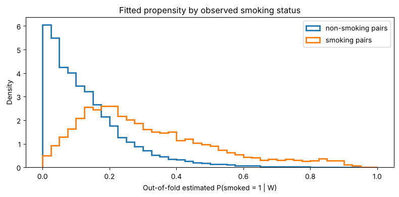
../_images/3a0199caf949ac5ac6275e397125c2bf8e3a1f8b5ea4ea14747f07bde0fc6afd.png

What this output tells you. The ATT needs non-smoking pairs at the background of each smoking pair. The largest fitted propensity is 0.9537, below the upper bound 0.975. The non-smoking pairs thin out at high propensities. Their 99% quantile is 0.5631, while 5% of the smoking pairs lie above 0.7450. The histogram shows the same pattern.

The lower ATT bound 0.025 clips 6,686 pairs: 6,581 non-smoking and 105 smoking. A non-smoking pair enters the update with the weight g/(1 − g), so these pairs carry little weight. The truncation curve repeats the targeting step at five bounds. The estimate moves from 0.00144 to 0.00150 across them. The bound therefore does not carry the estimate, although the support summary warns that it might.

The Kish / target value of 0.375 shows that the load of the ATT update concentrates on a minority of the pairs. The library reports this value as a description, not as a measure of precision. These values describe the fitted propensity model. They do not show the overlap of the true assignment mechanism.

9. Sensitivity to unmeasured confounding#

The no-unmeasured-confounding assumption cannot be tested. The omitted-variable bound of Chernozhukov, Cinelli, Newey, Sharma and Syrgkanis (2026) states how far a confounder of a given strength could move the estimate. Its strength cf_y is the share of the residual outcome variation that the confounder explains. Its strength cf_d measures how much the confounder adds to the weights of the ATT. The worst-case alignment is ρ = 1. Omitted-variable bounds defines each quantity.

The code first calibrates the strengths. It refits without mother’s education and marital status, the two confounders that section 3 identifies, and it reports their implied strengths. It then reads the bound at the benchmark strengths and at three larger values of cf_y.

benchmark = result.sensitivity.benchmark(
    covariates=("mother_education", "married"), estimand="att", random_state=SEED
)
print(benchmark.summary())
print()
rows = []
for cf_y in (benchmark.cf_y, 0.001, 0.005, 0.01):
    if cf_y == benchmark.cf_y:
        # The benchmark record supplies its own gains as cf_y and cf_d. rho stays 1.
        bound = result.sensitivity.omitted_confounding(estimand="att", benchmark=benchmark)
    else:
        bound = result.sensitivity.omitted_confounding(
            estimand="att", cf_y=cf_y, cf_d=benchmark.cf_d, rho=1.0
        )
    rows.append(
        {
            "cf_y": round(cf_y, 4),
            "bias bound": bound.bias,
            "bias-adjusted lower": bound.lower,
            "bias-adjusted upper": bound.upper,
            "95% lower": bound.ci_lower,
            "95% upper": bound.ci_upper,
        }
    )
print(f"cf_d from the benchmark: {benchmark.cf_d:.4f}; rho = 1")
print(pd.DataFrame(rows).round(5).to_string(index=False))

Benchmark for 'att' against ['mother_education', 'married']
------------------------------------------------
quantity  with covariates  without  
--------  ---------------  ---------
estimate  0.0014499        0.0022752
sigma^2   0.02722          0.027227 
nu^2      11.079           10.214   

implied cf_y = 0.0003, cf_d = 0.0848, rho = 0.3355
the estimate moved by +0.00082531 when these covariates were dropped

cf_d from the benchmark: 0.0848; rho = 1
  cf_y  bias bound  bias-adjusted lower  bias-adjusted upper  95% lower  95% upper
0.0003     0.00268             -0.00123              0.00413   -0.00556    0.00847
0.0010     0.00528             -0.00384              0.00673   -0.00817    0.01108
0.0050     0.01182             -0.01037              0.01327   -0.01471    0.01762
0.0100     0.01671             -0.01526              0.01816   -0.01962    0.02254

What this output tells you. Without education and marital status, the estimate moves from 0.0014499 to 0.0022752, a change of +0.00082531. The two covariates imply cf_y = 0.0003, cf_d = 0.0848, and ρ = 0.3355. The refit keeps the father’s education and the other covariates, which partly stand in for the two dropped ones. The implied strengths therefore measure what the two covariates add beyond the other covariates.

The outcome-side strength is small because the outcome is rare. The outcome model has an R² of 0.014, so chance explains most of the outcome variation.

`cf_y`	bias bound	bound with 95% confidence
0.0003 (the benchmark)	0.00268	[-0.00556, 0.00847]
0.0010	0.00528	[-0.00817, 0.01108]
0.0050	0.01182	[-0.01471, 0.01762]
0.0100	0.01671	[-0.01962, 0.02254]

Each row uses the benchmark cf_d and ρ = 1. The benchmark implies ρ = 0.3355, so ρ = 1 is conservative. At the benchmark strengths, the bias bound 0.00268 already exceeds the estimate. The upper end 0.00847 also exceeds the crude difference 0.0078. A missing confounder as strong as education and marital status could therefore hide an ATT as large as the crude difference. The bound also assumes a consistently estimated propensity, and the calibration flag of section 8 qualifies that.

10. A check for over-adjustment#

Three items of C can change during the pregnancy: alcohol use, diabetes, and lung, heart, or kidney disease. The certificate does not say whether they began before the pregnancy. If smoking affects one of them, adjustment for it removes part of the effect. The code refits the ATT without the three items and prints both estimates.

# Three items of C can change during the pregnancy, so smoking could affect them.
possibly_affected = ("alcohol", "diabetes", "lung_heart_kidney_disease")
without = result.sensitivity.benchmark(
    covariates=possibly_affected, estimand="att", random_state=SEED
)
print(f"ATT with the three items:    {without.psi_long:.4f}")
print(f"ATT without the three items: {without.psi_short:.4f}")
print(f"standard error of the ATT:   {att.std_error:.4f}")

ATT with the three items:    0.0014
ATT without the three items: 0.0022
standard error of the ATT:   0.0026

What this output tells you. Without the three items, the estimate moves from 0.0014 to 0.0022. The change is about a third of the standard error 0.0026. Its direction agrees with over-adjustment, and it also agrees with confounding by the three items. The data cannot separate these two explanations. Both estimates are small against their sampling error, so the choice does not change the reading of section 6.

Method evidence#

The fit on this page uses observed data, so no true value is known. The registered study in the table measures the estimator over repeated draws of a synthetic law. The study page gives its law, its nuisance models, and the result of each cell.

fit on this page	registered study	law of the study
Section 6, the ATT	Stacked point-treatment CV-TMLE	a synthetic law with a bounded continuous outcome

No registered study covers this Super Learner, three folds, a rare outcome, or 51,874 pairs.

The technical entry lists the evidence and the limits of the method.

What the analysis answers#

The estimate. Among same-sex twin pairs born alive in 1989–1991 to smoking mothers, in the reporting states and years, the first-year risk is 0.0427 per child as observed. The estimated risk had the mothers not smoked is 0.0412. The ATT is 0.0014, with a 95% interval of [-0.0037, 0.0066]. Among the 16,888 children of smoking pairs, that is 24 deaths, with a 95% interval from -63 to 112. The interval is an influence-curve Wald interval, with the pair as the unit.

What supports it. The targeting step solved its score equation. The estimate does not depend on the propensity bound. The estimator meets its coverage check on a simpler law.

What remains unverified. The graph and the choice of C are judgments. No unmeasured confounding, a correct record of smoking, no effect of smoking on C, and harmless selections are also judgments. Section 9 shows that a missing confounder as strong as education and marital status could hide an ATT as large as the crude difference.

What the analysis does not support.

It does not show that smoking is harmless to twins. The interval includes effects up to 0.0066, and the sensitivity bound admits larger ones.
It does not estimate the effect for singletons, for other years, or for the states that did not collect the item.
It does not support an effect estimate within birth-weight bands. Section 7 shows why such estimates mislead.
The gap between the crude difference and the ATT comes from one data set. It does not measure the confounding bias of other data sets.

Where to go next#

Point-treatment TMLE teaches the same estimator on a synthetic law with a known answer. CV-TMLE and cross-fitting shows why the nuisance predictions come from other folds. Results assessment describes each check of section 8.